
IFRAME SYNC
Labels
- Blog – Mathematics & Statistics
- Blog on math blogs
- Blog: Math and Life
- Cambridge Mathematics News
- Certain about uncertainty
- CUNYMath Blog
- Developmental Mathematics Revival!
- Discovering the Art of Mathematics blogs
- Engineering math blog
- Engineering Mathematics Tutorial
- Hot Weekly Questions - Mathematics Stack Exchange
- Institute for Mathematics and Computer Science
- Intellectual Mathematics
- Intersections -- Poetry with Mathematics
- math
- Math Blog
- Math Solutions
- Math with Bad Drawings
- mathbabe
- MathCancer Blog
- mathrecreation
- Maths & Physics News
- Mean Green Math
- MIND Research Institute Blog
- Mr. Shauver – Learner Educator
- Pennsylvania Mathematics Initiative
- Peter Cameron's Blog
- Problems in Mathematics
- RSM Blog
- Social Mathematics
- Solve My Maths
- SquareCirclez
- Stephen Wolfram Blog
- Surrey Mathematics Research Blog
- Tanya Khovanova's Math Blog
- Teaching High School Math
- The Aperiodical
- The Center of Math Blog
- What If Spreadsheet Math
- Wolfram Blog » Mathematics
- Wonder in Mathematics
- Yummy Math
Technology
Breaking News
July 2019
Aug 1, How to Check if the Function is One to One From its Graph
How to Check if the Function is One to One From its Graph
from Math Blog https://ift.tt/2MwkrEC
from Math Blog https://ift.tt/2MwkrEC
Aug 1, Inverse Functions Using Tables
Inverse Functions Using Tables
from Math Blog https://ift.tt/2LUZ1Bu
from Math Blog https://ift.tt/2LUZ1Bu
Math Instruction for Students Learning English
As of 2016, 4.9 million students — or 9.6% of students in U.S. public schools — were identified as English Language Learners (ELL), according to the National Center for Education Statistics. While different folks advocate using different terms to describe … Continue reading →
from Blog on math blogs https://ift.tt/316gN8z
from Blog on math blogs https://ift.tt/316gN8z
Jul 31, Relationship Between Domain and Range of a Function and its Inverse
Relationship Between Domain and Range of a Function and its Inverse
from Math Blog https://ift.tt/2YCw93b
from Math Blog https://ift.tt/2YCw93b
Are these two explicitly given $10 \times 10$ matrices similar over the integers? Or equivalently, are they shift equivalent over $\mathbb{Z}$?
Are the following two $10 \times 10$ matrices $$A = \left[ \begin {array}{cccccccccc} 0&1&0&0&1&0&0&0&0&0 \\ 0&0&1&0&0&1&0&0&0&0\\ 1&0&0&1&0 &0&1&0&0&0\\ 1&0&0&0&0&0&0&1&0&0 \\ 0&0&0&0&0&1&0&0&0&0\\ 0&0&0&0&0 &0&1&0&0&0\\ 0&0&0&0&1&0&0&1&0&0 \\ 0&0&0&0&1&0&0&0&1&0\\ 0&0&0&0&0 &0&0&1&1&1\\ 0&0&0&0&0&0&0&0&1&1\end {array} \right] $$
and
$$ B = \left[ \begin {array}{cccccccccc} 1&1&0&0&0&0&0&0&0&0 \\ 1&1&1&0&0&0&0&0&0&0\\ 0&1&0&0&0 &1&5&1&5&5\\ 0&0&0&0&1&0&6&10&5&1 \\ 0&0&1&0&0&1&6&6&10&5\\ 0&0&0&1&0 &0&10&5&1&5\\ 0&0&0&0&0&0&0&1&0&0 \\ 0&0&0&0&0&0&0&0&1&0\\ 0&0&0&0&0 &0&1&0&0&1\\ 0&0&0&0&0&0&1&0&0&0\end {array} \right] $$ similar over $\mathbb{Z}$?
I believe the answer to be no, but if the answer is yes, then these matrices form a counterexample to something (to be described below) I've been trying to prove recently in my PhD project. Let me give some context to my question by first indicating what I've tried and found out so far, and then giving some motivation and background after that.
What I've tried: Both matrices have characteristic polynomial $${t}^{10}-2\,{t}^{9}-{t}^{8}-{t}^{7}+2\,{t}^{6}+6\,{t}^{5}-{t}^{3}-4\,{ t}^{2}-2\,t+1,$$ and they both have the same Frobenius/Rational canonical form, this being just the companion matrix of said polynomial:
$$ F = \left[ \begin {array}{cccccccccc} 0&0&0&0&0&0&0&0&0&-1 \\ 1&0&0&0&0&0&0&0&0&2\\ 0&1&0&0&0 &0&0&0&0&4\\ 0&0&1&0&0&0&0&0&0&1 \\ 0&0&0&1&0&0&0&0&0&0\\ 0&0&0&0&1 &0&0&0&0&-6\\ 0&0&0&0&0&1&0&0&0&-2 \\ 0&0&0&0&0&0&1&0&0&1\\ 0&0&0&0&0 &0&0&1&0&1\\ 0&0&0&0&0&0&0&0&1&2\end {array} \right] $$ So we know that $A$ and $B$ are similar over $\mathbb{Q}$ (as they are both similar to $F$). I have actually been able to show that $A$ is similar to $F$ also over $\mathbb{Z}$. This was done using a "lucky" computer search: I ran through all size $10$ vectors $\vec v$ with entries in $\{-1,0,1\}$ and checked whether the matrix with columns $\vec v$, $A \vec v$, $\ldots$, $A^9 \vec v$ had determinant $\pm 1$. This was the case for a handful of $\vec v$'s, so these matrices witness the integral similarity of $A$ and $F$. The same search for $B$ did not yield any positive results though. I would like to try a search on a larger set of vectors, but this would require more computing power than I posess currently (being home for the summer holidays). If the matrices are not similar, this method will of course never give the answer though...
From the above we nevertheless have the following equivalent question: Are the matrices $B$ and $F$ above similar over $\mathbb{Z}$?
Another idea: Another idea I've had is to consider the matrices $A$ and $B$ (or $F$ and $B$) as matrices over the finite field $\mathbb{F}_p$ for various choices of the prime $p$. As this can be decided using the Frobenius form. If there is a $p$ for which the matrices are not similar over $\mathbb{F}_p$, then they are not similar over $\mathbb{Z}$ either. So that would settle it. However, if for some large $p$, $A$ and $B$ are similar over $\mathbb{F}_p$, I hope that a the transformation matrix witnessing this similarity also could work over $\mathbb{Z}$, because the $p$ is so large. This is just speculation though. My problem is that I'm not sure which software I could use to perform these finite field calculations effeciently. Any feedback on this is greatly appreciated!
Motivation: This part will be a bit brief/cryptic, in order to keep it short, so please just let me know if I should give more details on something.
This question has come out of my recent attempts to prove that shift equivalence implies flow equivalence for (certain) non-negative integral matrices and their associated shifts of finite type. The dynamical systems called shifts of finite type, which are associated to a non-negative integer matrix, are described in the introductory textbook "An Introduction to Symbolic Dynamics and Coding" by Douglas Lind and Brian Marcus. Shift equivalence of matrices and flow equivalence of shifts of finite type are also explained in the book (starting on pages 233 and 453).
For non-negative integer matrices which are irreducible (meaning that for each $i,j$ $A^n(i,j) > 0$ for some $n$), it is known that shift equivalence implies flow equivalence. This is because in the irreducible case there is a complete algebraic invariant in terms of the defining matrix which determines flow equivalence. And it is not hard to see that shift equivalence over $\mathbb{Z}$ (which is weaker than mere shift equivalence) preserves the invariant.
For reducible matrices, however, the invariant is a lot more complicated. So in this case it is an open problem whether shift equivalence (over $\mathbb{Z}$) implies flow equivalence. It is not clear at all whether shift equivalence preserves the invariant. There is a recent paper in another field which hints at this potentially being true, so that is why I've spent some time trying to prove it. After failing to prove it I started searching for counterexamples instead. There are counterexamples if one allows the matrices to have "cyclic components", meaning that one irreducible component is essentially a permutaton matrix, but this makes the shifts of finite type a bit "degenerate" in some sense, so I want to avoid that.
The way shift equivalence over $\mathbb{Z}$ connects with similarity over $\mathbb{Z}$ is that this is actually equivalent, for matrices with determinant $\pm 1$ (i.e. those which are invertible over $\mathbb{Z}$). This is the case for $A$ and $B$. The matrices $A$ and $B$ are constructed to not be flow equivalent. They both have a similar block structure which is a by-product of the construction (edit: see the comments for the block structure), but I have chosen to not get into that.
from Hot Weekly Questions - Mathematics Stack Exchange
The Best Joke I’ve Ever Written (according to my wife Taryn)
Here it is, the joke which forms the centerpiece of my marriage:
 (Please, hold your raucous applause.)
Oddly enough, this joke belongs to a micro-genre of “humor about failed transformations.”
For example, Taryn is also a big fan of this cartoon:

And back in the day, she was a staunch advocate of this video:
Help me out, folks. It’s her birthday next week. What are some other jokes playing on the concept of illogical or ill-conceived transformations?
from Math with Bad Drawings https://ift.tt/2MvXRMk
A junior with some bad anxiety and too many interests, trying to choose a Degree ideas
This might not be the best sub for this but I got some good answers on r/physics so I wanted to get more opinions. I don’t really wanna study pure mathematics, I like the technical aspect like Electrical and Computer engineering, but I’ve been told you don’t use a lot of math in the real world careers for this major. I thought about the sciences (Physics or Computer science) but those are harder jobs to get afterwards and idk what other jobs you can get with them. And then recently I’ve thinking about a business degree like Economics or Finance but I feel like I’ve been less prepared for it thus far and idk much about it. Software Developer was also on my list but there isn’t really a category for it.
In general I like solving problems (theoretical and real-world), Analysis, and Research. I have friend who does Operations Research (for the military) which sounds like it’d be a good job but he just happened to get the job as a physics major I’m not sure what the best way to get the job is or if that major is useful other ways.
[link] [comments]
from math https://ift.tt/33dchai
Asymptotic behaviour of a weird power series
Let $\varepsilon \in (0, 1)$ and consider the analytic function $$f(x) = \sum_{n=1}^\infty n^\varepsilon \frac{x^n}{n!}.$$ What is the order of growth of $f(x)$ as $x \to \infty$? From the basic inequality $1 \leqslant n^\varepsilon \leqslant n$ I deduced $$e^x - 1 < f(x) < xe^x$$ but I would like an asymptotic equivalence $$f(x) \sim g(x) e^x \qquad (x \to \infty)$$ where $g(x)$ is sufficiently familiar (e.g. a combination of $\log$s). How do I proceed?
from Hot Weekly Questions - Mathematics Stack Exchange
Any good theoric books for mathematic that you would recommend for a 15 years old?
So I want to develop my ability and knowledge regarding mathematics, but I don’t know where to start. If you have any good book idea that I could read(theory by preference). Just to say, we finished the year with second degree equations if that can help you.
[link] [comments]
from math https://ift.tt/2GEoIlz
What Are You Working On?
This recurring thread will be for general discussion on whatever math-related topics you have been or will be working on over the week/weekend. This can be anything from math-related arts and crafts, what you've been learning in class, books/papers you're reading, to preparing for a conference. All types and levels of mathematics are welcomed!
[link] [comments]
from math https://ift.tt/31ctEWV
Are original movies better than their sequels?
 We've gathered some data on movie ratings and their sequels and asked students to analyze the data, decide on some analysis and debate (with their mathematical data) which are better ... the original movies or their sequels.
Students see what they can conclude from various types of graphs and consider what size random sampling of movies and their sequels is an adequate, representative population of movies. This is a very open ended activity that will allow 6th or 7th graders to conduct data analysis at one level: measures of central tendency & variability, box plots,histograms ect. While high school students might work with greater sophistication, doing some of the same work as middle school students, but extending their work to consider the spread of the data, normal curve & standard deviation. The last question in the activity gets at sample size. This is your opportunity to discuss sample size and random sampling and certainty in your data analysis.
The activity: Sequel2019.pdf
CCSS: 6.SP.1, 6.SP.2, 6.SP.3, 6.SP.4, 6.SP.5, 7.SP.1, 7.SP.3, 7.SP.4,HSS.ID.A.1,HSS.ID.A.2, HSS.ID.A.3, HSS.ID.A.4, HSS.IC.A.1
For members we have an editable Word docx, an Excel sheet of the data and graphs, and solutions.
Sequel2019.docx Sequel2019.xlsx Sequel2019-solution.pdf
from Yummy Math
BCC at Birmingham, days 1-3
This week I am in Birmingham for the British Combinatorial Conference.
The organisation of the conference is outstanding. For one small example, yesterday, fifteen minutes before the Business Meeting was due to start, the Chairman noticed that we didn’t have the minutes of the previous Business Meeting to approve. The Secretary had the file on a laptop, and before the meeting started we had fifty printed copies to distribute.
After the excitement about ADE last week, these diagrams reappeared twice in the first couple of days, Hendrik Van Maldeghem (who talked about geometrical and combinatorial constructions of buildings) showed us all the crystallographic Coxeter–Dynkin diagrams. In a completely different context, Alexander Gavrilyuk mentioned the fact that connected simple graphs with spectral radius at most 2 are the ADE diagrams and the extended ADE diagrams. He attributed this to Smith (1969) and Lemmens and Seidel (1973). I think it would be not unjust to say that this result was part of the classification of the complex simple Lie algebras by Cartan and Killing in the last decade of the nineteenth century. That aside, Alexander was extending this to directed graphs, using a Hermitian adjacency matrix with entries 1 if there are arcs both ways between two vertices, while single arcs from v to w have i (the complex fourth root of 1) in position (v,w) and −i in position (w,v). This had been done by Guo and Mohar, but some small corrections were necessary; he used results of Greaves and McKee to achieve these. (As a footnote to this, it seems to be that to use τ, a complex 6th root of unity, in place of i would be more natural, since the sum of τ and its complex conjugate is 1 rather than 0.)
In fact, for the graph case, much more is known: the graphs whose greatest eigenvalue is at most 2 are the ADE diagrams and their extensions, but the graphs whose least eigenvalue is at least −2 can also be described.
The conference featured mini-symposia, and I organised one on “Designs and Finite Geometries”, which in my opinion has had some beautiful talks so far, from Ian Wanless on plexes in Latin squares, Rosemary Bailey on designs related to the Sylvester graphs (and the wrong turnings on the way to finding them), Peter Keevash on his and others’ results on existence of designs (including the fact that estimates for the number of Steiner systems, asymptotic in the logarithm, are now available, and hinting that he had constructions of large sets of Steiner systems for large admissible orders), and Moura Paterson on authentication schemes.
One of the most exciting talks was by Igor Pak. He has formulae, and good asymptotic estimates, for the numbers of standard Young tableaux for various skew Young diagrams. This was a mix of all kinds of things, including counting linear extensions of posets, rhombus tilings, plane partitions, counting disjoint paths, Vershik’s limiting tableau shapes, and a remarkable formula of Coxeter, which (if I copied it correctly) says
Σ(φn/n2) cos(2πn/5) = π2/100
(the sum over all positive integers n.)
Coxeter’s discovery of this formula was based on the existence of the 600-cell (a regular polytope in 4 dimensions) and some spherical geometry. As far as I can tell, the formula was not actually used in the talk, but the philosophy of it led to some of the things that came later.
Two things about the talk were a pity. First, there was no paper in the Proceedings. (In the history of the BCC, it has happened a few times that a speaker provided no talk; indeed I was the editor of the first “published-in-advance” volume, at Royal Holloway in 1975, where I failed to get papers from either Conway or Kasteleyn.) So I am unable to check these details. Second, Igor started in a bit of a rush, and some things were not clearly explained. For example, I think some nodding acquaintance with Plancherel measure is needed to make sense of the Vershik asympotic shape of a random Young diagram, and I didn’t find that in the talk. But it was so full of amazing stuff that it is perhaps churlish to complain.
Apart from these I will be very selective in my reporting. One contributed talk I really enjoyed was by Natasha Dobrinen, on the Ramsey theory of Henson’s homogeneous Kn-free graphs, which included a description of them in terms of trees. It went part rather fast (the talks were only 20 minutes), but I wonder whether this leads to a probabilistic approach to Henson’s graph. I have reported before how I laboured over this, and how Anatoly Vershik explained to me his construction with Petrov in a leisurely afternoon in Penderel’s Oak in London – a construction which is clearly related to the topic of graphons, the subject of Dan Král’s talk.
Then there was a sequence of three nice talks on quite different topics, but all related to permutations (in the combinatorial rather than the group-theoretic sense). Simon Blackburn proved a nice asymptotic result about random permutations for the uniform measure. At the end, Robert Johnson asked whether there were similar results for other measures. This was because Robert’s talk, which was next, was able to prove some of the results for wider classes of measures, though not for the Boltzmann measure, which he gave as an open problem. Then Fred Galvin talked. One of his results was that, far from being monotonic, the sequence of coefficients (excluding the constant term) in the independent set polynomial of a graph with independence number m can be any permutation of {1,…m}. This suggested to me another interesting measure on permutations. Choose n much larger than m, and choose a random graph on n vertices with independence number m; this induces a probability measure on the permutations. Does this measure tend to a limit as n→∞? If so, this could claim to be a “natural” measure on permutations. Fred thought this was an interesting question.
Any ideas?
We had a reception in the remarkable Barber Institute of Fine Arts. Guided tours of the gallery were offered. We went upstairs, and the first picture we saw was René Magritte’s famous picture “The flavour of tears”. Tuesday was the concert, and apart from having to move to a different room because the piano hadn’t been unlocked, we had a remarkable evening’s entertainment; there are several outstanding pianists at the conference. Today is the excursion, to the Museum of Black Country Living; but I have work to do …
from Peter Cameron's Blog https://ift.tt/2Kt7JnJ
Recursion . . . in a life . . . in a poem . . .
The New Yorker offers a rich variety of poetry and in their print issue of 22 July 2019 they give a poem that I love: "Sentence" -- by Tadeusz Dabroswski (translated from the Polish by Antonia Lloyd-Jones) plays with two meanings of the word "sentence" and also embodies the concept of recursion -- so important in mathematics. Below I offer the opening lines; at this link may be found the entire poem (both a print version and an audio recording).
Sentence by Tadeusz Dąbrowski
It’s as if you’d woken in a locked cell and found
in your pocket a slip of paper, and on it a single sentence
in a language you don’t know.
Read more »
from Intersections -- Poetry with Mathematics
Sentence by Tadeusz Dąbrowski
It’s as if you’d woken in a locked cell and found
in your pocket a slip of paper, and on it a single sentence
in a language you don’t know.
Read more »
from Intersections -- Poetry with Mathematics
Prove that if $x$ is odd, then $x^2$ is odd
Prove that if $x$ is odd, then $x^2$ is odd
Suppose $x$ is odd. Dividing $x^2$ by 2, we get: $$\frac{x^2}{2} = x \cdot \frac{x}{2}$$ $\frac{x}{2}$ can be rewritten as $\frac{x}{2} = a + 0.5$ where $a \in \mathbb Z$. Now, $x\cdot\frac{x}{2}$ can be rewritten as:
$$x\cdot\frac{x}{2} = x(a+0.5) = xa + \frac{x}{2}$$
$xa \in \mathbb Z$ and $\frac{x}{2} \notin \mathbb Z$, hence $xa + \frac{x}{2}$ is not a integer. And since $xa + \frac{x}{2} = \frac{x^2}{2}$, it follows that $x^2$ is not divisible by two, and thus $x^2$ is odd.
Is it correct?
from Hot Weekly Questions - Mathematics Stack Exchange
Examining $\int_0^1 \left(\frac{x - 1}{\ln(x)} \right)^n\:dx$
I'm currently working on the following family of integrals: \begin{equation} I_n = \int_0^1 \left(\frac{x - 1}{\ln(x)} \right)^n\:dx \end{equation} Where $n \in \mathbb{N}$. I employed Feynman's Trick coupled with the Dominated Convergence Theorem and Leibniz's Integral Rule. In doing so, I introduced the following function: \begin{equation} J_n(t) = \int_0^1 \left(\frac{x^t - 1}{\ln(x)} \right)^n\:dx \end{equation} Where $0 \leq t \leq 1 \subset \mathbb{R}$. With some fairly easy steps, I end up with the following ODE: \begin{equation} J_n^n(t) = (-1)^n \sum_{j = 1}^n {n \choose j} (-1)^j \frac{j^n}{jt + 1} \nonumber \end{equation} Where $J_n^k(t)$ is the $k$-th derivative of $J_n(t)$ with the conditions $J_n^k(0) = 0$ for $ 0 \leq k \leq n$. As such, to resolve $J_n(t)$ I need to integrate $J_n^n(t)$ $n$ times whilst applying the initial conditions. Although I can do it for any fixed $n$, I'm yet to be able to generalise it for any $n$. I was wondering if anyone has working with this type of ODE and if so, is there any preferable ways to approach it?
Initially I thought that using Laplace Transforms would be ideal as in applying it to $J_n^n(t)$ all terms would be removed given the initial condition. This felt apart as the Laplace Transform of $\frac{1}{t + a}$ is a nasty Special Function to work with.
So, to repeat, is there an approach people can recommend?
For anyone who may be interested, here is my work on this integral:
In this section, I would like to address the following family of integrals: \begin{equation} I_n = \int_0^1 \left( \frac{x - 1}{\ln(x)} \right)^n \:dx \nonumber \end{equation}0 To begin with, consider the case when $n = 1$: \begin{equation} I_1 = \int_0^1 \frac{x - 1}{\ln(x)}\:dx \nonumber \end{equation} Here we introduce the function: \begin{equation} J_1(t) = \int_0^1 \frac{x^t - 1}{\ln(x)}\:dx \nonumber \end{equation} We observe that $I_1 = J_1(1)$ and $J_1(0) = 0$. Here we employ Leibniz's Integral Rule and differentiate under the curve with respect to $t$: \begin{equation} J_1'(t) = \int_0^1 \frac{\frac{d}{dt}\left[x^t - 1 \right]}{\ln(x)}\:dx = \int_0^1 \frac{\ln(x)x^t}{\ln(x)}\:dx = \int_0^1 x^t \:dx = \left[ \frac{x^{t +1}}{t + 1}\right]_0^1 = \frac{1}{t + 1} \nonumber \end{equation} We now integrate with respect to $t$: \begin{equation} J_1(t) = \int \frac{1}{t + 1} \:dt = \ln\left|t + 1 \right| + C \nonumber \end{equation} Where $C$ is the constant of integration. To resolve $C$ we employ $J_1(0) = 0$: \begin{equation} J_1(0) = 0 = \ln\left|0 + 1\right| + C \rightarrow C = 0 \nonumber \end{equation} Thus, \begin{equation} J_1(t) = \ln\left|t + 1\right| \nonumber \end{equation} We now resolve $I_1$ using $I_1 = J_1(1)$: \begin{equation} I_1 = J_1(1) = \ln\left|1 + 1\right| = \ln\left|2\right| \nonumber \end{equation} The question I have is: Can this approach be used for other or all values of $n$?. To address this, I will proceed by applying the same method to $n = 2$: \begin{equation} I_2 = \int_0^1 \frac{\left(x - 1 \right)^2}{\ln^2(x)}\:dx \nonumber \end{equation} We introduce the function: \begin{equation} J_2(t) = \int_0^1 \frac{\left( x^t - 1\right)^2}{\ln^2(x)}\:dx \nonumber \end{equation} We observe that $I_2 = J_2(1)$ and $J_2(0) = 0$. We proceed here by employ Leibniz's Integral Rule and differentiate under the curve with respect to $t$: \begin{equation} J_2'(t) = \int_0^1 \frac{\frac{d}{dt}\left[\left(x^t - 1\right)^2 \right]}{\ln^2(x)}\:dx = \int_0^1 \frac{2\left(x^t - 1\right)\ln(x)x^t}{\ln^2(x)}\:dx = 2 \int_0^1 \frac{x^t\left(x^t - 1\right)}{\ln(x)}\:dx \nonumber \end{equation} We observe that $J_2'(0) = 0$. We now differentiate again with respect to $t$: \begin{equation} J_2''(t) = 2\int_0^1 \frac{\ln(x)x^t\cdot \left(x^t - 1\right) + x^t \cdot \ln(x)x^t}{\ln(x)}\:dx = 2\int_0^1 2x^{2t} - x^t \:dx = 2\left[\frac{2x^{2t + 1}}{2t + 1 } - \frac{x^{t + 1}}{t + 1} \right]_0^1 = 2\left[\frac{2}{2t + 1} - \frac{1}{t + 1}\right] \nonumber \end{equation} We now integrate with respect to $t$: \begin{equation} J_2'(t) = 2\int \frac{2}{2t + 1} - \frac{1}{t + 1} \:dt =2\bigg[ \ln\left|2t + 1\right| - \ln\left|t + 1\right| \bigg] + C \nonumber \end{equation} Where $C$ is the constant of integration. To resolve $C$, we use $J_2'(0) = 0$: \begin{equation} J_2'(0) = 0 = 2\bigg[\ln\left|2\cdot 0 + 1\right| - \ln\left|0 + 1\right|\bigg] + C = 0 + C \rightarrow C = 0 \nonumber \end{equation} Thus, \begin{equation} J_2'(t) = 2\bigg[\ln\left|2t + 1\right| - \ln\left|t + 1\right|\bigg] \nonumber \nonumber \end{equation} We now integrate again with respect to $t$: \begin{equation} J_2(t) = 2\int \ln\left|2t + 1\right| - \ln\left|t + 1\right| \:dt = 2\bigg[\left(\frac{2t + 1}{2}\right)\bigg[ \ln\left|2t + 1\right| - 1 \bigg] - \bigg[ \left(t + 1\right)\ln\left|t + 1\right| - t \bigg] \bigg] + D \nonumber \end{equation} Where $D$ is the constant of integration. To resolve $D$ we use the condition $J_2(0) = 0$: \begin{equation} J_2(0) = 0 = 2\bigg[\left(\frac{2\cdot 0 + 1}{2}\right)\bigg[ \ln\left|2\cdot 0 + 1\right| - 1 \bigg] - \bigg[ \left(0 + 1\right)\ln\left|0 + 1\right| - 0 \bigg]\bigg] + D = -1+ D \rightarrow D = 1 \nonumber \end{equation} Thus, \begin{equation} J_2(t) = 2\bigg[\left(\frac{2t + 1}{2}\right)\bigg[ \ln\left|2t + 1\right| - 1 \bigg] - \bigg[ \left(t + 1\right)\ln\left|t + 1\right| - t \bigg]\bigg] + 1 \nonumber = \left(2t + 1\right)\ln\left|2t + 1\right| -2\left(t + 1\right)\ln\left|t + 1\right| \nonumber \end{equation} Thus, we now may resolve $I_2$ using $I_2 = J_2(1)$: \begin{equation} I_2 = J_2(1) = \left( 2\cdot 1 + 1\right)\ln\left|2\cdot 1 + 1\right| -2 \left(1 + 1\right)\ln\left|1 + 1\right| = 3\ln(3) -4\ln(2) \nonumber \end{equation} Here I will attempt to resolve the integral in it's general form. I will employ the same approach as for $n = 1, 2$ and introduce the function: \begin{equation} J_n(t) = \int_0^1 \frac{\left(x^t - 1 \right)^n}{\ln^n(x)}\:dx \nonumber \end{equation} We observe that $I_n = J_n(1)$ and $J_n(0) = 0$. We begin by expanding the integrand's numerator using the Binomail Expansion: \begin{equation} J_n(t) = \int_0^1 \frac{\sum_{j = 0}^n { n \choose j} \left(x^t\right)^j \left(-1 \right)^{n - j}}{\ln^n(x)}\:dx = (-1)^n \sum_{j = 0}^n {n \choose j} (-1)^j \int_0^1 \frac{x^{jt}}{\ln^n(x)}\:dx \nonumber \end{equation} Taking the same approach as before, we now employ Leibniz's Integral Rule and differentiate $n$ times under the curve with respect to $t$: \begin{equation} J_n^n(t) = (-1)^n \sum_{j = 0}^n {n \choose j} (-1)^j \int_0^1 \frac{\frac{d^n}{dt^n}\left[x^{jt}\right]}{\ln^n(x)}\:dx \nonumber \end{equation} Here we note: \begin{equation} \frac{d^n}{dt^n}\left[x^{jt}\right] = j^n \ln^n(x)x^{jt} \nonumber \end{equation}, Noting that for $j= 0$, the derivative is $0$. Thus, \begin{equation} J_n^n(t) = (-1)^n \sum_{j = 1}^n {n \choose j} (-1)^j \int_0^1 \frac{j^n \ln^n(x)x^{jt}}{\ln^n(x)}\:dx = (-1)^n \sum_{j = 1}^n {n \choose j} (-1)^j j^n \int_0^1 x^{jt}\:dx = (-1)^n \sum_{j = 1}^n {n \choose j} (-1)^j \frac{j^n}{jt + 1} \nonumber \end{equation} Where $J_n^k(0) = 0$ for $k = 0,\dots, n$.
from Hot Weekly Questions - Mathematics Stack Exchange
Jul 31, Finding Inverse of a Function for Particular Value
Finding Inverse of a Function for Particular Value
from Math Blog https://ift.tt/2YhW4la
from Math Blog https://ift.tt/2YhW4la
Jul 31, Finding Inverse of a Function
Finding Inverse of a Function
from Math Blog https://ift.tt/2Yqpzkf
from Math Blog https://ift.tt/2Yqpzkf
Solve in positive integers $8xy-x-y=z^2$
I deduced that $8z^2+1=(8x-1)(8y-1)$, but then I don't know what to do.
from Hot Weekly Questions - Mathematics Stack Exchange
Microdosing and mathematics
Has anyone here microdosed on LSD before? I've heard of engineers in Silicon Valley doing it because it supposedly increases your output and creativity. If anyone has any experience microdosing and doing mathematics please share your observations, I'm really curious.
[link] [comments]
from math https://ift.tt/316QDmg
Proving a reversed AM-HM inequality
Problem:
Given $n \ge 3$, $a_i \ge 1$ for $i \in \{1, 2, \dots, n\}$. Prove the following inequality: $$(a_1+a_2+\dots +a_n) (\frac{1}{a_1}+\frac{1}{a_2} + \dots +\frac{1}{a_n}) \le n^2+\sum_{1\le i<j\le n}|a_i-a_j|.$$
This inequality seems like a reversed form of AM-HM inequality (which states that $\operatorname{LHS}\ge n^2$). I know that Kantorovich inequality is of the same direction, but that is not helpful. I tried to apply Cauchy–Schwarz inequality, but failed.
Thanks for any help.
from Hot Weekly Questions - Mathematics Stack Exchange
Chaotic permutation with repetition
Is there a generalyzed formula of chaotic permutation with repetition of elements in the sequence? For example: how many anagrams of mathematics there are in witch none of the letters assume their right position?
[link] [comments]
from math https://ift.tt/319lyOP
Why is set theory at the foundation of mathematics?
As the title says, it has always struck me as odd that these rather complex structures are used to define the most basic of logic and arithmetic. Even operations on sets like union, intersection, etc. are actually complicated operations, and anyone who has done any programming will know that this is the case. Is it possible that we're getting ahead of ourselves when it comes to the fundamentals of mathematics?
[link] [comments]
from math https://ift.tt/2K3xWtI
A finite order restriction of a Fredholm operator is also a Fredholm operator.
Let $A:D(A) \subseteq H \to H$ and $B:D(B) \subseteq H \to H$ be closed linear operators on a Hilbert space $H$ such that $A$ is a finite order extension of $B$, that is, $B \subseteq A$ and $\mbox{dim } D(A)/D(B) < \infty$. I need to show that if $\lambda \notin \sigma(A)$ and $\lambda I-A$ is a Fredholm operator, then $\lambda I-B$ is also a Fredholm operator.
There is a hint: Since $A$ is a finite order extension of $B$, the difference of the resolvents is of finite order.
But, I don't know how can I use the hint. Can I say that $\lambda \notin \sigma(B)$?
My attempt
Since $\lambda I-A$ is a Fredholm operator, by definition of a Fredholm operator we know that $\mbox{dim} (\ker (\lambda I-A))<\infty$, $\mbox{dim} (H/R(\lambda I-A))<\infty$ and the range $R(\lambda I-A)$ of $\lambda I-A$ is closed in $H$. From here we get that $\mbox{dim} (\ker (\lambda I-B))<\infty$.
Thank you for any help you can privide me.
from Hot Weekly Questions - Mathematics Stack Exchange
MIND Blog Rewind: July 2019
Each month here on the MIND blog we are sharing the stories of how our organization, our partners, and educators across the country are advancing the mission to mathematically equip all students to solve the world’s most challenging problems. We’re also sharing resources for educators and students, and covering some of the exciting events we’re taking part in across the country.
There’s a lot to talk about, so we want to make sure you don’t miss any of it. Welcome to the MIND Blog Rewind, where each month we’ll be recapping some of the great content coming out of MIND and our community in the past month. Here’s your roundup of stories from July 2019:

Alesha Arp shared some strategies for avoiding the “summer slide” by fueling students' curiosity over the summer months. She recounts her own experiences with her daughter, as well as lessons learned from being an educator and a Senior UX Researcher here at MIND.
Kelsey Skaggs recapped a very busy week for MIND at ISTE 2019. From the collaboration with our partner Cisco, to thought leadership sessions featuring our own Brandon Smith and Ki Karou, to the epic meeting between JiJi Cisco’s Huti, it was an event to remember.
Our new Content Specialist Jolene Haley wrote about MIND’s Independence Day celebration, which capped off her first month at MIND. She reflected on the uniqueness of the culture we have here at MIND, and how our leadership team drives that culture.
EVP and Social Impact Director Karin Wu highlighted our recent Partner Advisory Forum, provided some insight into how just how passionate and committed our partners are, and how important their guidance is to MIND. She also shared a video recap of the event, that features our partners as well as co-founder and Chief R&D Office, Matthew Peterson!
Education Engagement Manager Calli Wright provided an overview of the exciting ST Math updates, features and resources that educators will see when they return for the upcoming school year.
Our Chief Data Science Officer Andrew Coulson returned to the Inside Our MIND podcast, this time to discuss the issue of statistical significance. He explains how one of the checks and balances in research has been misunderstood and misapplied to the extent that the research community is starting to move away from the term entirely.
We rounded out the success story out of Madison, Virgina month with a great success story out of Madison, Virgina. Principal Mike Coiner and Instructional Coach Jessi Almas from Madison Primary School share the secret to their growth in test scores, learning, and innovation with ST Math.
There was a little bit of something for everyone is this month’s roundup, so hopefully you found something that resonated with you. If you did, let us know! You can comment on the blog below, and you can share this (and all) of our blogs on your favorite social media channel by using the sharing buttons at the top of each post. And of course, you can subscribe to the blog if you haven't already using the email sign-up at the top of the main blog page. Thanks for reading!
from MIND Research Institute Blog https://ift.tt/2Ms47oz


Jul 30, Finding the Missing Value in Composition of Two Functions
Finding the Missing Value in Composition of Two Functions | Example problems with detailed steps
from Math Blog https://ift.tt/2MqO8Hd
from Math Blog https://ift.tt/2MqO8Hd
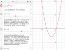
Do 3/8 (37.5%) of Quadratics Have No x-Intercepts?
I randomly had a thought about what proportion of quadratics don't have real x-intercepts. Initially I thought 33%, because 0,1,2 intercepts, then I thought that the proportion of 1 intercepts is infinitesimal. So I then thought 50%, as graphically half the quadratics would be above the x axis, the other half below.
If you put it into a list of (max,min) and (above,below): Minimum + Above = no x intercepts
Minimum + Below = 2 x intercepts
Maximum + Above = 2 x intercepts
Maximum + Below = no x intercepts.
Hence 50% right?
Well I simulated it using code. I randomised a, b and c, and output the discriminant. If it is less than 0, add 1 to a variable. Do this about 100000 times. Now divide the variable by 100000. I get numbers like this (37.5%$\pm$0.2).
I hypothesise that it averages 3/8.
Why?
Now I hypothesise there may be a fallacy to my approach of finding the 'proportion'. Fundamentally, it is the probability of getting a quadratic with no x intercepts. However, I am not sure.
EDIT: The range was from (-n,n), where n was 100000, or even higher.
from Hot Weekly Questions - Mathematics Stack Exchange
Jul 30, rank of matrix questions 3
Rank of Matrix Questions 3 | Definition and Example problems of finding rank of matrix
from Math Blog https://ift.tt/2YtnR1f
from Math Blog https://ift.tt/2YtnR1f
Jul 30, Evaluating the Value of Composition Function from the Given Functions
Evaluating the Value of Composition Function from the Given Functions | Solution with detailed steps
from Math Blog https://ift.tt/2ylHMRb
from Math Blog https://ift.tt/2ylHMRb
IntMath Newsletter: Eigenvectors, 3D solar system, graphics
30 Jul 2019
In this Newsletter:
1. New on IntMath: Eigenvalues and eigenvectors
2. Resources: Desmos and 3D simulator
3. Math in the news: News and science
4. Math movies: Graphics and addresses
5. Math puzzle: Tangent circles
6. Final thought: Culture
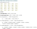
1. New on IntMath: Eigenvalues and eigenvectors
Eigenvectors are very important in many science and engineering fields, including compuer science. (Google's search algorithm is based on eigenvectors.) It was one of the many topics I learned about as a math student where I could find the answers, but I really had no idea what I'd found, what the concept really meant, or what they were good for.
I wrote some new pages incorporating interactive applets which I hope gives the reader a better idea of what this interesting topic is all about. (It's usually taught at university level, but the mathematics involved is not that challenging - mostly multiplying and adding.)
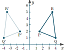 |
On this page we see how multiplying by a matrix can achieve the kind of transformations graphics artists and robot designers use a lot, including reflection, rotation, skew (shear), scaling and displacement. |
The applet on this next page allows you to explore the physical meaning and geometric interpretation of eigenvalues and eigenvectors.
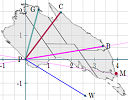 |
I've used stretching of a map of my home country to show how transformations achieved by matrix multiplication can be replaced with much simpler scalar multiplication (which is a key idea of this topic). |
Like most matrix operations, it's very easy to make simple mistakes when calculating eigenvalues and eigenvectors.
 |
This calculator allows you to check your work, and/or to explore what happens with eigenvectors for everything from 2x2 and 3x3 up to 9x9-size matrices. |
You may also be interested in:
How to find eigenvalues and eigenvectors? (outlining the algebraic steps for finding them - this was the only part I learned at university).
Applications of eigenvalues and eigenvectors (which includes a highly simplified description of how Google search works).
2. Resources
(a) Using Desmos to create learning resources
Here's a recent tweet by teacher Liz Caffrey:
 |
Check out how one of my students uses the graphing calculator to take notes! She sets up and saves a new graph each day. Here are her notes from our notice/wonder on standard form of quadratics! I never would have thought of doing this. |
I know from my own experience how much richer my understanding of topics is after I've created similar interactive explorations. Doing it with Desmos is really quite easy, and I encourage you (whether student or teacher) to give it a go. You don't need a lot in the way of programming skills.
(b) Harmony of the spheres
This is a 3D simulation of the solar system, built on an "open source gravity simulator".
It also has some "What-if" scenarios. This example shows what would happen if Earth actually orbitted Saturn:
 |
You can drag left-righ, up-down to explore and use the mouse wheel to zoom. Press the "Play" button at the top to animate the scene. |
You can also change the physics parameters, and add masses. It's very nicely done. (Probably best on a laptop.)
3. Math in the news: News and science
Last week marked the 50th anniversary of the moon landings. This was an extraordinary human achievement, but the misguided belief that it was all a hoax continues to grow, fuelled by ignorant people (and bots) through social media. Where and how we find our news, and how we critically examine the sources and conclusions, becomes increasingly important as the growth of fake news has the potential to rip apart our societies.
(a) How do we find out what's happening?
In the US, more people get their news from social media than traditional news sources, while in other countries it's the reverse. See a short summary: Where do people find news on their smartphones?
From the original Digital News Report, by Reuters and University of Oxford: Executive Summary and Key Findings of the 2019 Report
(b) What do we know about science?
Those of us involved in science education would like to think most students graduate with a reasonable general knowledge of the various branches of science, and will have a good grounding in how science actually works. But it appears that is not always the case.
The (US) National Science Board's Science and Engineering Indicators 2018 makes for some sobering reading.
Science and Technology: Public Attitudes and Understanding
Here's a sample of the misunderstandings gleaned from the results of various quizzes.
- Antibiotics kill viruses (which is false): 50% or more got it wrong in most countries
- Human beings developed from earlier species of animals (true): 30 to 50% got it wrong
- Astrology is scientific (false): around 40% (US) thought it was true
- Understanding experimental design: over 50% got it wrong in most countries
No wonder we have the growth of drug-resistant superbugs, rampant species destruction, and climate change deniers.
4. Math Movies
(a) The simple genius of a good graphic
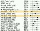 |
Data visualization is an increasingly important item in everyone's skill set these days. Information designer Tommy McCall outlines the evolution of charts and diagrams with plenty of interesting examples. |
(b) A precise, three-word address for every place on Earth
When I first arrived in Japan where I lived for 4 years, I was amazed at how different their address system was compared to what Iwas used to. Rather than sequential numbers (usually odd on one side and even on the other) along roads, the Japanese system is built around regions and sub-regions of a suburb.
So I found the pretext of this next talk quite interesting.
 |
Many houses do not have any kind of address system, and to find anyone, you need to rely on local knowledge. Chris Sheldrick has an interesting solution - use three-word addresses! |
I like the basic concept, but surely numbers are more universal? Wouldn't addresses based on latitude and longitude make more sense, especially as that's how our phones know where we are already?
5. Math puzzles
The puzzle in the last IntMath Newsletter asked about the possible dimensions of 2 pencils.
A correct answer with sufficient reasons was submitted by Georgios. Special mention to Nicola who worked on a generalized solution involving circles and ellipses, which she explored using Desmos.
New math puzzle: Tangent circles
Circles that are "mutually tangent" touch at one point only. We have 3 such circles, with centers P, Q, R and radii p, q, r respectively. We are given the lengths PQ = 15, QR = 21 and PQ = 14. Find p, q and r.
You can leave your response here.
6. Final thought - culture

Pangolin (image credit)
Living in different countries gives you fresh insights about culture. A lot of the cultural practices that seemed vital to our existence have faded as time goes on, and others we question due to their environmental impacts. While they may not have had much effect hundreds of years ago when there were less people in the world, perhaps some aspects of the following don't make a lot of sense any more?
- Buying SUVs for suburban runabouts
- Living in large houses a long way from work
- Eating whale meat
- Burning paper in the Hungry Ghost Festival
- Consuming rhino horn, pangolin scales and shark fin
- Buying ivory carvings
- Wearing baby seal furs
Maintaining the traditions while minimizing their impacts is surely the best way to move forward.
Until next time, enjoy whatever you learn.
Related posts:
- IntMath Newsletter: Vector graphics, regression manga In this Newsletter: 0. Notice any problems on IntMath? 1....
- IntMath Newsletter: Solar vision, GeoGebraTube In this Newsletter: 1. Math teacher's solar vision 2. GeoGebraTube...
- IntMath Newsletter: Conic sections, resources, Ramanujan In this Newsletter: 1. Conic sections interactive applet 2. Resources...
- IntMath Newsletter: Domain, range, Azure, Riemann In this Newsletter: 1. New applet: Domain and range exploration...
from SquareCirclez https://ift.tt/2yoU9Mg
via IFTTT
Jul 30, Evaluate the Indicated Value of Composition Function From the Table
Evaluate the Indicated Value of Composition Function From the Table
from Math Blog https://ift.tt/331Of1C
from Math Blog https://ift.tt/331Of1C
Paper of Cesare Tronci to appear in Proceedings of the Royal Society of London

from Surrey Mathematics Research Blog https://ift.tt/2K4uvmI
Jul 30, Reflecting a Graph in the Horizontal or Vertical Axis
Reflecting a Graph in the Horizontal or Vertical Axis|Definition and examples
from Math Blog https://ift.tt/2K4tgny
from Math Blog https://ift.tt/2K4tgny
Jul 30, Stretch a Graph Vertical or Horizontal Examples
Stretch a Graph Vertical or Horizontal Examples
from Math Blog https://ift.tt/2ymc7yS
from Math Blog https://ift.tt/2ymc7yS
How does one start a literature search for a paper?
I just had a cool idea (and proof) for an interesting way to implement a common imperative algorithm that commonly has tight constraints can have those tight constraints loosened considerably and it still behave quite well with a pretty trivial invariant.
I'm 'just' a software developer who is a big fan of mathematics. I have no idea how to go about seeing if this is novel, nor how to pursue publication.
What do!?
Thanks guys, HomeBrewingCoder
[link] [comments]
from math https://ift.tt/331laDN
Examples of sets which are not obviously sets
In my (limited) experience, it is usually easy to see when something is large enough to be a proper class, by constructing an element of the class for every set.
However, sometimes such a proper class has lots of redundant information, so we consider it modulo some equivalence relation. This way, in some cases, we end up with something small enough to be (represented by) an actual set!
Motivating example: The Witt group $W(F)$
(actually, we don't care about the group structure, I'm sorry)
Let $F$ be a field. Let $$ W(F) := \{(V, q)\ \text{quadratic}\ F\!-\!\text{vector spaces}\}/\sim $$ Where $(V, q)\sim (W, r)$ if there exist metabolic (i.e., hyperbolic plus degenerate) spaces $E_1, E_2$ such that $(V, q)\perp E_1 \simeq (W, r)\perp E_2$, where $(V, q)\perp (W,r) = (V\oplus W, (v,w)\mapsto q(v)+r(w))$.
Then $W(F)$ is a set has a set of representatives.
When I first learned this, this was not at all obvious to me.
(To be honest, I only vaguely recall this, and am not too sure of the technical details. The gist of this was however, that we only consider finite-dimensional vector spaces in the first place, which allow only for a finite number of non-equivalent quadratic forms, and even after that, most of those can be seen to be equivalent to a quadratic space of lower dimension by adding elements to make a large portion look hyperbolic)
Question
So, in a similar spirit to this question:
What are other non-obvious examples of sets, e.g. proper classes being “quotiented” to a set?
from Hot Weekly Questions - Mathematics Stack Exchange
What is beauty? Is mathematics beautiful?
My thoughts have been turned to the beauty of mathematics by stumbling onto a very fine article, "Beauty Bare: The Sonnet Form, Geometry and Aesthetics," by Matthew Chiasson and Janine Rogers -- published in 2009 in the Journal of Literature and Science and available online here.
The article opens with this quote from A Mathematician's Apology (see p. 14) by G. H. Hardy: Beauty is the first test: there is no permanent place
in the world for ugly mathematics.
Read more »
from Intersections -- Poetry with Mathematics
The article opens with this quote from A Mathematician's Apology (see p. 14) by G. H. Hardy: Beauty is the first test: there is no permanent place
in the world for ugly mathematics.
Today I'm puzzling over what "beauty" means . . .
Read more »
from Intersections -- Poetry with Mathematics
In a compact metric space, if we keep adding closed balls centered on boundary, do we always cover the entire space?
Let $X$ be a compact connected metric space, and let $W_1=B(x,r)$ denote the closed metric ball centered at $x\in X$ with radius $r$. We recursively define $W_{k+1}=W_k \cup B(y,r)$, where $y$ denote a point on the boundary of $W_k$ and $B(y,r)$ is not contained in $W_k$.
Is it true that there always exist $n>0$ such that $W_n=X$ for some $n$?
If not, is there any additional requirement that can make this true?
from Hot Weekly Questions - Mathematics Stack Exchange
What Are You Working On?
This recurring thread will be for general discussion on whatever math-related topics you have been or will be working on over the week/weekend. This can be anything from math-related arts and crafts, what you've been learning in class, books/papers you're reading, to preparing for a conference. All types and levels of mathematics are welcomed!
[link] [comments]
from math https://ift.tt/2Yqp9pF
Print Quality in Previous Editions of "What is Mathematics?" by Courant and Robbins?
Looking at the current 1996, second edition of this classic book it appears the print quality is fairly poor. It features blurred text, variable sized text, low quality diagrams, and sub/superscripts that are illegible. I have read that it is sourced from a photocopy.
I was wondering if owners of the past versions of the first edition, particularly the affordable 1979 edition, have this problem also, or are more readable?
Thanks for your help.
[link] [comments]
from math https://ift.tt/32Z3ZCA
Let $f: \mathbb{R}^n \rightarrow \mathbb{R}$. Is the set of points at which $f$ is differentiable a Borel set?
Let $f: \mathbb{R}^n \rightarrow \mathbb{R}$ be a function. Is the set of points at which $f$ is differentiable a Borel set?
The answer is "yes" for $n=1$, even for arbitrary $f$ (not assumed to be measurable).
But what happens for $n>1$? The proof for $n=1$ (refer Characterization of sets of differentiability) does not seem to generalize easily to higher dimensions.
(The motivation for asking this question came from the Rademacher's theorem, which states that any Lipschitz map $f:\mathbb{R}^n \rightarrow \mathbb{R}$ is differentiable almost everywhere. I was wondering if the points where $f$ is not differentiable forms a Borel set. Therefore, if the solution to the original question seems obscure, please feel free to help me with partial results, especially for the Lipschitz case.)
from Hot Weekly Questions - Mathematics Stack Exchange
Integral $ \int_0^\infty \frac{\ln x}{(x+c)(x-1)} dx$
I've been trying to solve the following integral for days now.
$$P = \int_0^\infty \frac{\ln(x)}{(x+c)(x-1)} dx$$
with $c > 0$. I figured out (numerically, by accident) that if $c = 1$, then $P = \pi^2/4$. But why? And more importantly: what's the general solution of $P$, for given $c$? I tried partial fraction expansions, Taylor polynomials for $ln(x)$ and more, but nothing seems to work. I can't even figure out where the $\pi^2/4$ comes from.
(Background: for a hobby project I'm building a machine learning algorithm that predicts sports match scores. Somehow the breaking point is this integral, so solving it would get things moving again.)
from Hot Weekly Questions - Mathematics Stack Exchange
Absolute formulas with high complexity
It is a standard result that $\Sigma_1^{\mathsf{ZF}}$-formulas are upward absolute between $\mathsf{ZF}$ $\in$-models, while $\Pi_1^{\mathsf{ZF}}$-formulas are downward absolute between $\mathsf{ZF}$ $\in$-models, so in particular $\Delta_1^{\mathsf{ZF}}$-formulas are absolute between $\mathsf{ZF}$ $\in$-models.
This is also sharp, there are some stronger results ($\Pi_2^{\mathsf{ZF}}$-formulas are $H(\kappa)$-$V$-downward absolute for an uncountable $\kappa$), but in general it's not hard to construct $\Sigma_2^{\mathsf{ZF}}$, $\Pi_2^{\mathsf{ZF}}$ and $\Delta_2^{\mathsf{ZF}}$-formulas for which the appropriate absoluteness result fails.
Is there a simple way to construct, given $n\in\Bbb N$, a formula $\varphi$ such that $\varphi$ is $\Delta_n^{\mathsf{ZF}}$ (and not equivalent to a simpler formula) and $\varphi$ is absolute between $\mathsf{ZF}$ $\in$-models?
from Hot Weekly Questions - Mathematics Stack Exchange
Engaging students: Introducing the number e
In my capstone class for future secondary math teachers, I ask my students to come up with ideas for engaging their students with different topics in the secondary mathematics curriculum. In other words, the point of the assignment was not to devise a full-blown lesson plan on this topic. Instead, I asked my students to […]
from Mean Green Math
from Mean Green Math
Jul 29, Shifting the Graph Right or Left Examples
Shifting the Graph Right or Left Examples
from Math Blog https://ift.tt/2JZezlv
from Math Blog https://ift.tt/2JZezlv
Jul 29, Shifting Graph Up and Down Examples
Shifting Graph Up and Down Examples
from Math Blog https://ift.tt/2YsooN0
from Math Blog https://ift.tt/2YsooN0
Area under a parametric curve – How to get that?
Area under a parametric curve. Hello friends, today I’ll talk about the area under a parametric curve. Have a look!! The area under a parametric curve Suppose and are the parametric equations of a curve. Then the area bounded by the curve, the -axis and the ordinates and will be Now I’ll solve...
The post Area under a parametric curve – How to get that? appeared first on Engineering math blog.
from Engineering math blog https://ift.tt/2MlX4O1
Is this just a lucky proof for the Basel problem?
I'll begin by showing that: $$\int_0^\infty \frac{\ln x}{x^2-1}dx=\int_0^1\frac{\ln x}{x^2-1}dx+\underbrace{\int_1^\infty\frac{\ln x}{x^2-1}dx}_{x\to \frac{1}{x}}=2\int_0^1 \frac{\ln x}{x^2-1}dx$$$$=-2\sum_{n=0}^\infty \int_0^1 x^{2n}\ln xdx=2\sum_{n=0}^\infty \frac{1}{(2n+1)^2}=\frac32\sum_{n=1}^\infty \frac{1}{n^2}$$
On the other hand, from here we have the following results: $$\int_0^\infty \frac{\ln x}{(x+a)(x+b)}dx{=\frac{\ln(ab)}{2}\frac{\ln\left(\frac{a}{b}\right)}{a-b}=\frac{\ln^2a -\ln^2 b}{2(a-b)}}\tag 1$$
$${\int_0^\infty \frac{\ln x}{(x+a)(x-1)}dx=\frac{\ln^2 a+\pi^2}{2(a+1)}} \tag 2$$
Obviously by putting $a=1$ in $(2)$ we get: $$\int_0^\infty \frac{\ln x}{x^2-1}dx=\frac{\pi^2}{4}\Rightarrow \sum_{n=1}^\infty \frac{1}{n^2}=\frac{\pi^2}{6}$$ However this is circular, since in the linked post, to prove $(2)$ one used this result.
Let's just say that I was brave enough and plugged $b=-1$ in $(1)$ to get: $$\int_0^\infty \frac{\ln x}{(x+a)(x-1)}dx=\frac{\ln^2a -\ln^2 (-1)}{2(a-(-1))}=\frac{\ln^2 a+\pi^2 }{2(a+1)}$$ We already know that this is true, but let's ignore $(2)$.
Hopefully my question isn't that stupid, (tbh it looks like a fluke) but
Can someone prove (or disprove) rigorously that we are allowed to plug in $b=-1$ in order to get the correct result?
Or alternatively can someone prove the result in $(2)$ starting from the result in $(1)$ by a different method?
The main motivation behind this, is that to prove $(1)$ we only need one substitution and a proof for Basel problem becomes quite nice and elementary.
from Hot Weekly Questions - Mathematics Stack Exchange
In which field (besides $\mathbb{R}$) is every symmetric matrix potentially diagonalizable?
In which field (besides the well-known $\mathbb{R}$) is every symmetric matrix potentially diagonalizable? A matrix is potentially diagonalizable in a field $F$ if it is diagonalizable in the algebraic closure of $F$.
It appears to me that the fields $\mathbb{F}_2$ and $\mathbb{C}$ do not have this property. What about other finite fields?
from Hot Weekly Questions - Mathematics Stack Exchange
Jul 28, Ratios rates tables and graphs worksheet
Ratios rates tables and graphs worksheet
from Math Blog https://ift.tt/2LLGcR8
from Math Blog https://ift.tt/2LLGcR8
Jul 28, Inverse relation
Inverse relation
from Math Blog https://ift.tt/313BOk2
from Math Blog https://ift.tt/313BOk2
Is cardinality continuous?
Let the underlying set theory be ZFC. Let $x_1 \subseteq x_2 \subseteq \dots$ and $y_1 \subseteq y_2 \subseteq \dots$ be ascending sequences of sets such that, for every $n \in \{1,2,\dots\}$, $|x_n| = |y_n|$. Is it the case that $\big|\cup_{n =1}^{\infty}x_n\big| = \big|\cup_{n =1}^{\infty}y_n\big|$? If this is not generally true, is it possible to characterize all those—or at least some interesting—cases for which this does hold? Is there a standard terminology for these cases? Can this be generalized to transfinite sequences? Does the answer change if we require that the sequences be strictly increasing, i.e. for every $n \in \{1,2,\dots\}$, $x_n \subsetneq x_{n+1}$ and $y_n \subsetneq y_{n+1}$?
from Hot Weekly Questions - Mathematics Stack Exchange
Jul 28, Algebraic Manipulation Problems
Algebraic Manipulation Problems
from Math Blog https://ift.tt/2Zf7nHr
from Math Blog https://ift.tt/2Zf7nHr
Is there a number field of degree n whose ring of integers is a unique factorization domain?
For every $n$, can we find a number field of degree $n$ whose ring of integers is a unique factorization domain?
As a Dedekind domain is a UFD iff it is a PID, this is equivalent to asking the following: For every $n$, can we find a number field of degree $n$ with class number 1.
from Hot Weekly Questions - Mathematics Stack Exchange
Good books
I love the Brian Greene physics books. Is there one similar on mathematics?
[link] [comments]
from math https://ift.tt/2Y7ZF5f
What is the maximum of $\sum_{k=1}^{\infty} (-1)^k(^kx)$?
During my testing of the series $\sum\limits_{k=1}^{n} (-1)^k(^kx)$, I found that the sum converges to two limits when $n \to \infty$, for $e^{-e} \lt x \le e^{1/e}$ and oscillates between depending on whether $n$ is even or odd.
Here, $^kx$ is tetration. The notation $^kx$ is the same as $x^{x^{x^{....}}}$, which is the application of exponentiation $k-1$ times. Ex. $^3x=x^{x^x}$.
Questions:
$(1)$ What is the maximum and minimum of $\lim\limits_{n\to \infty}\sum\limits_{k=1}^{n} (-1)^k(^kx)$ for even $n$?
$(2)$ What is the maximum and minimum of $\lim\limits_{n\to \infty}\sum\limits_{k=1}^{n} (-1)^k(^kx)$ for odd $n$?
Edit:
Also during my testing in PARI, I observed that the sum seems to converge to two values only in the domain of $e^{-e} \lt x \le e^{1/e}$. I think the reason for this maybe is that, since $^{\infty}x$ converges only for $e^{-e} \lt x \le e^{1/e}$, the sum also converges for the same domain. I would appreciate if someone could explain why the sum converges only for $e^{-e} \lt x \le e^{1/e}$.
from Hot Weekly Questions - Mathematics Stack Exchange
How do I master the GMAT syllabus?
First of all, I thank you for your time and help! I am sorry for any grammatical mistakes. In 3 months I will be giving an exam called CAT (Common admission Test), which is basically GMAT but for Indian b schools. The topics are - Arithmetic and Data Interpretation, Algebra, Geometry, and Modern math (set theory, permutation combination, and probability). Although, the syllabus is similar to GMAT, the CAT asks more advanced questions. I have completed the lectures of Geometry and Arithmetic +DI, but I don't practice enough (I don't know how to). Geometry is one of my biggest hurdles. Every question is totally new! I think that I have understood a concept (After learning one) but I can't apply it. I have always been weak in mathematics. What should I do to get a decent score in these examinations? How should I master these topics?
[link] [comments]
from math https://ift.tt/2ZhOraK
Jul 28, Distance Between Two Points Calculator
Distance Between Two Points Calculator
from Math Blog https://ift.tt/2LKsA8U
from Math Blog https://ift.tt/2LKsA8U
An exercise from Apostol's book
I am trying to solve following problem from Apostol's Mathematical Analysis. The problem could be very trivial, but I am not getting clue for it.
Let $\{a_n\}$ be a sequence of real numbers in $[-2,2]$ such that $$|a_{n+2}-a_{n+1}|\le \frac{1}{8} |a_{n+1}^2-a_n^2| \,\,\,\, \mbox{ for all } n\ge 1.$$ Prove that $\{a_n\}$ is convergent.
Q. Any hint for solving this? (I was not getting the restrictions of interval and the factor $\frac{1}{8}$).
My try: since $a_i\in [-2,2]$ so $a_i^2\in [0,4]$. Thus, $|a_{n+1}^2-a_n^2|\le 4$ and so $|a_{n+2}-a_{n+1}|\le \frac{1}{2}$. After this, I couldn't proceed.
Any HINT is sufficient.
from Hot Weekly Questions - Mathematics Stack Exchange
Bears Ears revisited

Clicking on this image will show it larger in a new window.
There is some beautiful land in Utah that was changed last year from federally protected land to Utah overseen land. The buttes of Bears Ears (shown above) and the surrounding territory contain over 100,000 archaeological sites and are sacred land to many American Tribes.
Ed Robinson, the Utah state director of the Bureau of Land Management, says that these changes will allow for off-road vehicles, hunting, shooting, fishing and other recreational uses.
Do you think that recreation was the point of this change? Was this sacred land needed to allow for population expansion, recreation, or what? Let your students examine the data and make their own conclusions.
Warning: This discussion could get politically active.
Below is our slide show of some of the beauty and ancient ruins of the original Bears Ears Monument. (Best viewed full screen.)
The activity: BearsEarsNationalMonument.pdf
CCSS: 6.RP.A, 7.RP.A, HSF.IF.C, HSS.ID.A, MP3
For members we have an editable Word docx and solutions.
BearsEarsNationalMonument.docx BearsEarsNationalMonument-solution.pdf
from Yummy Math
Jul 28, Transpose Matrix Calculator
Transpose Matrix Calculator
from Math Blog https://ift.tt/2yl7wx7
from Math Blog https://ift.tt/2yl7wx7
Jul 28, Squared Matrix Calculator
Squared Matrix Calculator
from Math Blog https://ift.tt/2Mib0bI
from Math Blog https://ift.tt/2Mib0bI
Education in the Age of Industry 4.0: conference in Lincoln
Dr Matt Watkins from School of Maths & Physics of University of Lincoln will give a talk “Connecting Academia to Industrial Focussed Machine Learning” at the Industry–Academic Collaboration Conference in Lincoln Education in the Age of Industry 4.0 on Monday 29th July 2019. The conference is supported by the funding from the Office for Students secured by the University of Lincoln.

Research highlights the difficulties that employers are having recruiting people with the right digital skills and places the responsibility for increasing supply of digital skills with government, universities and business. In January 2018 the University of Lincoln secured funding from the Office for Students to co-create a suite of modules and curricula to equip our graduates and workplace learners to meet the digitalisation challenges that our industrial partners face now and in the future. This one day national conference is an opportunity to share University of Lincoln findings from the Industrial Digitalisation Project and to hear from industry and other educational establishments on their strategies to meet the workforce challenges of Industry 4.0.
Agenda:
10.30 Registration
10.55 Welcome Prof Mary Stuart – Vice Chancellor University of Lincoln
11.00 Martin Collison – Director of Collison & Associates Ltd. Using Automation & Digitalisation to Create Higher Quality Jobs in the Food Chain
11.25 Dr Kamaran Fathulla – Senior Lecturer in Industrial Digitalisation – University of Lincoln. Embedding Industry 4.0 in the Curriculum
11.40 Lynda Crosby – Careers and Employability University of Lincoln. Lincoln Award Achievements
11.50 Dr Tim Jackson – Reader and the Undergraduate Admissions Tutor in the Department of Electronic, Electrical and Systems Engineering University of Birmingham. Creation of a single system to support the development of higher level skills in students
12.15 Session 1 Q & A
12.30 – 13.30 Lunch
13.30 Melanie Armstrong – Senior Advisor, Manufacturing Technology Centre. Digital Skills for Manufacturing
13.55 Chris Thompson, Sarah Edwards – Anglian Water. Changing Mind Set
14.05 Dr Matt Watkins School of Maths & Physics University of Lincoln. Connecting Academia to Industrial Focussed Machine Learning
14.15 Dr Clare Watson – MACE Computing. Curriculum with Digital Media Archives
14.25 Dr Steve Jones – Connected Curriculum Lead Working at Liverpool John Moores University for Siemens. Multi-Disciplinary Engineer for the 21st Century – Project Outcomes
14.50 Session 2 Q & A
15.05- 15.25 Coffee break
15.25 Jake Norman – OAL. Group Application of Digital Technologies in Food Manufacturing
15.50 Gyles Lingwood – Director of Education College of Arts – University of Lincoln. Challenge-based Learning in the Arts; Employability and Creativity
16.10 Session 3 Q & A
16.25 Conference close – Prof Libby John Pro Vice Chancellor / Head of College of Science
16.30 Wine reception and networking opportunity
from Maths & Physics News
copyrighted to mathematicianadda.com. Powered by Blogger.